Monday, July 20, 2020

Peak-Gap-Peak feature presentation for Exo3 conference

I am presenting the Peak-Gap-Peak feature to the Exo3 Conference.

I place some supporting links here, highlighted by linking my explanation of "How to See These Features Yourself":


1. How to obtain a histogram showing the gap in period space, as shown in Taylor 2019:
Go to http://exoplanets.org/plots and choose "Advanced" and "Histogram Plot". 
Enter "Per" into the data field to to histogram the period (per), 
Click log scale to bin by log period.
Click "Add Filter" upon which to do the binning.
Then enter this filter into the "Filter" field (it does not matter if you name the filter):
MSINI[mjupiter] > 0.0 && FE > 0.00 && PER[day] > 1 && PER[day] < 5001 && STARDISCMETH = 'RV' && TEFF[k] > 4500 && TEFF[k] < 6500 && LOGG > 4.00 && !BINARY && ECC < 01.20 && DATE < 2016
Then click "Configure Histogram" to adjust the size and placement of the bins:
Choose Logarithmic Bins
Enter the Bin Factor: 1.169576076
Enter the “Min”imum to be 0.938
Enter a max of 5e+3
These were to get boundaries of four bins to fall at the period of 923.8 and 493.7 days.
The “deep” (zero objects) part of the gap goes down to 653.22 days, which is 0.55 of the gap in log period, or a little more than the two longer period bins.
From 653.22 days to the boundary of the short period pileup at 493.7 days, there are six objects in what we call the “shallow” gap.
Then the double-peak separated by a gap from Figure 1 of Taylor 2019 pops right out!

If you choose to see the histogram binned on the equilibrium temperature based on multiplying the semi-major axis “A” with the dependence on stellar mass of M^(-0.5), then replace using the period in the X-axis with
A*MSTAR^(-0.5)


2. How to view the scatter plot that shows the gap shifting in semi-major axis with stellar mass, with a slope in log space of -1/2
Choose “Advanced” and “Scatter Plot”
Click "Add Filter"
Then enter this filter into the "Filter" field:
MSTAR[msun] < 1.29 && MSTAR[msun] > 0.7 && PER[day] > 0 && A[au] > 0.0 && A < 3.5 && MSINI[mjupiter] > 0.0 && NCOMP >= 1 && FE >= 0.00 && STARDISCMETH = 'RV' && TEFF[k] > 4500 && TEFF[k] < 10500 && LOGG > 0.20 && (!BINARY || STAR = 'HD 34445') && ECC < 01.20 && DATE < 2019
The choice of Mstar and A are made to focus in on the gap.
To see how the gap ends with objects having Mstar of 1.29 Msun in the gap, choose Mstar < 2.3
To see the lines as straight, (with a slope of -½ in logarithmic space), choose a minimum A above zero (i.e. A>0.1), and then you can choose logarithmic bins.
Note that for one planet of HD 34445 the star is incorrectly labeled as a binary star, so the planets of this star are included regardless.


Thursday, August 23, 2018

Briefly About My Research on Planets and How I Present Doing Science

What could be a more exciting way to use all the new measurements of planets than to find new patterns in their distributions? Planets have been my passionate study since childhood, so now I am studying the distribution of exoplanet parameters. 

I have found new patterns in the counts per (logarithmic) period of planets that depend on how much iron is in the star, for planets of stars that are ``sunlike'' as described by their surface gravity and whether the star is alone or has a stellar companion. This follows my finding that in more than one period range, the orbits of such planets of ``sunlike-stars'' at have higher eccentricity if the star has more iron, but there is a period range where the orbits of planets of low iron stars have especially high eccentricities such that this ``eccentricity-iron'' correlation goes away in this range.

My other planets research has been to observe exoplanets to confirm their discovery and measure their parameters. With one other astronomer, I started a program of observing planets and measuring their parameters. Our group has grown this program to be an important part of several projects, and our group now included as being a major player in confirming TESS planets. 

I enjoy presenting my work to many professional and private audiences. 

I currently live between Hong Kong and Cottonwood, Arizona, though have lately been limited more to staying in Hong Kong. I enjoy being in Asia where I enjoy learning to speak and getting laughed at in two dialects of Chinese. I am active in several forms of public speaking including comedy and storytelling, where I include science as a primary topic. 

Tuesday, August 21, 2018

Crowdfunding to present new discovery of gap in exoplanets in Vienna

I have discovering on a gap in the distribution of exoplanets that I have prepared to present at a major conference, so I am crowdfunding on GoFundMe.com:
https://www.gofundme.com/battle-for-belonging

I hope to go to the 2018 August International Astronomical Union meeting in Vienna, or if not, the 2019 January American Astronomical Society (AAS) meeting in Seattle. 


Monday, January 8, 2018

Crowdfunding for 2018 January astronomy conference


This post was from 2018 January while I was attending the American Astronomical Society (AAS) meeting in Washington, DC. The post is being updated to campaign for attending either the 2018 August International Astronomical Union meeting in Vienna, or the 2019 January AAS meeting in Seattle. 

Due to changes by the crowdfunding company Indiegogo in no longer supporting Generosity.com, I have moved my crowdfunding site to
The link below no long works.

I am crowdfunding for support to present my discovery!

Read about my campaign for support for me to participate in astronomy at the crowdfunding site below (run by Generosity.com, a division of Indiegogo.com):

(2018 January Crowdfunding site to Indiegogo/Generosity for "Battle for Belonging" was here)

I made small donations available for you to show your support, but every expression large or small helps persuade larger donors whether crowdfunders or the observatories to whom I apply for jobs.
Even if you cannot support me there, I would be grateful for supportive comments here!

I have come to the astronomy conference to present my exoplanet discovery and to present my efforts to participate in astronomy. I was also accepted to perform a standup comedy routine. We will see how much the astronomy community supports the participation of everyone who has been contributing.

Please leave a comment of support for my persistence to be involved and included!

All expressions of support for participation are appreciated!

Sunday, November 20, 2016

Petition to Democratic Electors to change your vote to lead to the Electoral College choosing an alternative

Update: This petition has gone live! 
Please sign it: 
(https://www.change.org/p/electoral-college-electors-electors-unite-behind-a-choice-who-can-win-to-not-choose-an-unqualified-president)


I I leave the post from yesterday:

Please help me edit my petition to change who the electoral college chooses for President. Please help me get the best written petition possible.

My petition could work because it is directed first at Democrat electors. It is not certain to fail as are the efforts to persuade Republican electors to vote for Hillary Clinton. Please do not debate me over whether this could never work or is somehow improper: The point is that it is worth trying to get the electoral college to produce a different choice by convincing Democratic electors that there is nothing wrong and nothing disparaging to Ms. Clinton about coming together to offer up a new choice that perhaps enough Republican electors might change their votes.


I seek editing suggestions (but not debate) on the following text:


We petition all electors to come together to select a leader who can unify our country. We petition Democratic electors to take the lead by declaring their vote to select a different Republican to become President. This is the only chance to encourage Republican electors to vote for a leader that a real majority of Americans can support. This is the best way to protest the setup where she who gets the most votes is kept from winning. We petition electors to perform the duty that those who wrote the constitution gave you: Reject the selection of an unqualified President.
We encourage Hillary Clinton to tell her electors that they are free to vote for a candidate that can win the current setup. Changing their vote is not voting against her. Do not accept that after getting the most votes she is assigned fewer electors. The Electoral College can only send one message that counts. Our petition is a response from the people to keep America great and keep America together.
We petition as voters who may have wanted Hillary Clinton to win, as citizens who showed opposition by voting for third candidates, or even as citizens who regret voting for Donald J Trump.
We petition Democratic electors do change their votes to support reform of the procedure of choosing Presidents. Send a message of rejecting the flaws of the current formula of choosing electors as a flawed count that ignores who received the most votes. Your action is required to prevent an undemocratic formula from choosing the wrong winner yet again. The biggest honor you could give to citizens who voted for Hillary Clinton would be to offer her the opportunity to suggest which Republican would be the best alternative to selecting Donald J. Trump, but given that she may feel bound by recent tradition, we ask you to collaborate among yourselves.
Some Democratic electors have suggested suitable candidates that their Republican colleagues could choose instead of Donald J. Trump. We petition that you do not merely encourage other electors change their votes to one of these alternatives. We petition you to do so yourselves. Say you did it in response to the people.
We petition leaders to perform your constitutional duty of rejecting an unqualified candidate who is being chosen not by the most votes but by an undemocratic count of the votes where some votes count more than others.

We petition electors to work together to support the same qualified candidate who could bring the country together and show respect to the world. We need a leader who can America keep the great leader it has long been.

I plan this to be the first of three petitions, to provide another petition for citizens of the world to express their voice that the U.S. choose a suitable leader who cares about the people of the world and the health of the earth’s climate. 

The purpose of the third petition is to place questions on the petition website of the whitehouse.gov, to address that the government lacks an appropriate petition website such that the first two petitions must be presented on a private site such as change.org. I am afraid that the whitehouse.gov site would remove a petition advocating for a change in the selection of a presidential candidate, but feel that some constitutional questions such as whether electors could do this, and whether candidates who do not obtain the highest number of electoral candidates can say they release their electors. I think to receive a Whitehouse reply even only that the constitution allows electors to vote however they want and are not bound by tradition of being a rubber stamp body would give encouragement to this effort.

I believe the text already expresses fairly well what I hoped it would, but this is a serious effort, so I choose to open it to a wider audience for a very short time before posting it.

Monday, June 6, 2016

Rings and Gaps Everywhere?: Do the Same Planet Formation Patterns Happen at the Same Periods?

Rings and gaps found in disks from Saturn's rings to protoplanetary disks.

How are planets arranged? Disks, of course. Disks are everywhere in the universe, from Saturn's rings to galaxies, but also planetary systems appear to usually come arranged in disks. Centuries ago, astronomers were guessing that planets were formed in disks. Long before we could see any disks forming planets, Laplace pretty much got it right that planets form from disks of dust and gas. Now, new telescopes are finally observing disks where planet formation is likely taking place, in disks called proto-planetary disks (PPDs).

What is often the main features of disks? Gaps and rings, of course. Saturn's rings are not uniform, but come with bright rings of more material, and dark gaps of less material. Now that PPDs are presumably being observed, many are found to have gaps in them. The recent result by ALMA showing the disk material in TW Hydrae, the nearest PPD, is not the first to find a gap in a PPD (Andrews et al., 2016). Our solar system also has a gap in its distribution of planets, with a wide space between Mars and Jupiter where there is no major planet.

So are there gaps in the arrangements of other solar systems? Certainly there would be in multiplanet systems, but could there also be gaps in the arrangements of planetary systems in general? A region where planets do not form?

There certainly are ``rings,'' such as the ``three-day'' pileups of giant planets with periods a little over three days, and the ``1 AU pileup'' of planets with distances from the star, called ``semi-major axes,'' of over 1 AU (the sun to earth distance). There have also been found regions of fewer planets close in to the star, referred to as valleys or deserts.

Now I present a dramatically deep gap a little further out, where since Taylor (2013) I have presented how the pileup past 1 AU is, when looking at planets hosted by stars more rich in iron than the sun but otherwise mostly sunlike, is actually two pileups separated by a surprisingly wide and deep gap. Though I first found a gap of ``fewer planets'' in 2013, in 2014 I found if I select only sunlike single stars, cutting out evolved stars and stars with stellar companions, there are actually zero planets in the current dataset with periods from 656 to 923 days. 


Fig. 1. Artists concept of the protoplanetary disk (PPD) around the star TW Hyadrae (TW Hya). Credit: NAOJ.

Fig. 2. A synthesized image of the submillimeter (radio) emission from the TW Hya disk from Andrews et. al (2016) and inset zooming into the center shows gap and ring structure in this PPD. 
Fig. 3 Gaps and many smaller rings make up the rings of Saturn.


Features in the planet distribution

We show that similarly there are more detailed features than just the short and long period pileups that are obvious in the distribution of planets. We first show the full counts of planets, and then narrow our selection of planets to find peaks and gaps in the population of planets hosted by sunlike stars that have richer iron abundance than the sun. We describe there how the binning was chosen to best show the gap and peaks. We list a couple of conventions: We want to use the best sample for the broadest range of periods, so we use the sample of planets found by radial velocity (RV) here. It is too hard for other methods to probe the region of a few AU: the detection efficiency falls too much for transiting planets, but this range is too close to the star to be observed by direct imaging. Good counts of planets exist for 429 ``RV planets'' up to periods of 5000 days, so we ignore the spotty findings of planets with periods beyond 5000 days. Finally, we refer to the planet plus its host star plus orbit collectively as an ``object,'' where the eccentricity of an ``object'' means the eccentricity of the orbit, while the iron abundance of an ``object'' is the iron abundance of the star, and ``iron-poor'' (rich) objects are those hosted by stars with poorer (rich) iron abundance than the sun (or other value if specified).


The first histogram, Fig. 4, shows all the periods of 429 planet orbits found by radial velocity up to the end of 2015 as compiled by exoplanets.org with periods up to 5000 days. The 429 are separated into 149 ``iron-poor'' and 280 iron-rich objects (149 and 280 planets hosted by stars with less than/the same and more iron abundance than the sun respectively). Here we already see some structure appearing in the iron-rich object population: though both populations are clearly composed in part by broad peaks centered at periods a little under 1000 days, there are two peaks in the iron rich population.

When the binned counts of all 429 planets, or all RV objects, found by this one method are counted by logarithmic period up to period of 5000 days and are shown together as in Fig. 4, we see that there appear to be a shorter period pileup and a longer period broad pileup. The shorter period pileup was one of the first findings made from the early discoveries of exoplanets, and has since been associated with iron-rich objects (Dawson & Murray-Clay, 2013, hereafter DM13), that is, planets of stars with higher iron abundance than the sun. The longer period pileup has long been expected because planet formation was expected to much more readily occur at a distance from the star beyond a ``snow-line'' far enough from the heat of the star that condensation can occur. Indeed, we see these pileups, but  it is uncertain whether there are more detailed features beyond statistical fluctuations. There are smaller ups and downs in the counts that could be worth investigating for whether there could be variations that are significant.

Fig. 4. The number distribution by period of all 429 planets found by radial velocity (RV) by the end of 2016, with periods up to 5000 days (since the statistic cut off beyond that). It appears that there is a single ``1 AU'' pileup at periods from one year to 1000 days. Though the double peak bracketing a gap pattern is visible here, it looks like random jitter rather than the strong feature that it is when a more focused sample is chosen.

Separating the counts of iron-poor from iron-rich objects as in Fig. 5 shows the short period peak to be a feature of iron-rich objects, as found by DM13. The separated collections of iron-poor and rich objects have been shown to be different populations with different distributions. Below, we show that these populations do indeed have different distinct features in the number count by period. We have also begun discussing the eccentricity distribution by period. We find features separate out more distinctly by period than by semi-major axis, likely because the period adjusts some to change in stellar mass. We find features separate out more distinctly by period than by semi-major axis, likely because the period adjusts some to change in stellar mass. A plot of planets orbiting smaller stellar mass stars shows the peak is at shorter periods. The peak in lower stellar mass systems at shorter periods could cover up a gap that in higher mass occurs the same range of period.
Fig. 5. The number distribution by period of all 429 planets as in the previous figure but this time divided into two populations, with red denoting those 280 objects whose stars are more iron-abundant than the sun (which we will call ``iron-rich'' and in astronomer's notation written [Fe/H] > 0), and blue denoting those 149 objects whose stars are iron-poor relative to the sun (``iron-poor''; in astronomer's notation written [Fe/H] <= 0).The double peak bracketing a gap pattern is more visible here, in the iron-rich population, but it still could be taken as random features.
In Fig. 5 the longer period peak in the iron-rich population begins to divide into two peaks, which when we restrict our counting to the 243 ``sunlike'' objects in Fig. 6, this shows that the space in between the two peaks includes at least one gap of zero planets next to a sharply rising ``longer period'' peak. These 243 planets have been chosen for being hosted by stars that are sunlike in temperature, surface gravity, and in being single stars (not having a stellar companion as follows: only objects with effective temperature (of the star) ``Teff'' which was chosen to be 4500 to 6500 K, or roughly within 1000 K of 5772 K, the Teff  of the sun, and the strength of the surface gravity of at least 10000 cm/sec2, which in astronomy jargon means requiring that ``log g'' is greater than 4.0, compared to the solar log g of 4.4. We do not at this time cut objects with different stellar masses due to their small numbers, though may do so in the future.

The bins size and placement was chosen to best show the two peaks in the ``beyond 1 AU pileup'' and the gap in between them. We were able to choose as bin boundaries the boundary between the short period peak and the gap, and the boundary between the gap and the long period peak. We took a bin boundary just beyond the longest period of the short period peak of 493.4 days, choosing on the left side of the gap a bin boundary of 494 days, or 2.69 in log period of 493.4, and we took a bin boundary just shortward of the shortest period in the longer period peak of 923.8 days or 2.97 in log period, choosing on the right side of the gap a bin boundary at 923.5 days. There is a span of 0.27 in log period space, a factor of 1.87, from the period of 493.4 to 923.8 days. The choice of four bins between these two chosen periods allows the most reasonable presentation of detail that appears to be real, without having too much statistical fluctuation that appears in smaller bins. The ratio between each bin, called the ``bin factor'' on exoplanets.org, is then 1.17, which is in 0.067 in ``log 10 period space.'' Though there were only two bins in between the gap in Taylor (2013), we show below that detail may be apparent having the smaller binsize. 

It appears that there could be structure in the gap in between the double peaks, in the form of a small gap separated from a larger gap by a small pileup: All of the six planets in between the two peaks have periods in between 567 and 653 days, a distance of 0.061 in log period space which is small enough to fit into one of the bins that are of width 0.067, but this pileup starts after a small gap slightly smaller than a bin, a gap also spanning 0.061 in log period space. So the pileup goes from 0.22 to 0.44 of the fractional distance in between the two peaks. The pileup then is situated just slightly shortward of the 2nd bin, such that the first planet period falls in the first bin.  To show the gap/pileup/gap features, in Fig. 7 a smaller binsize (``bin factor'') of 1.17 corresponding to a distance in log 10 period of 0.067 is taken, and the same 243 objects as in Fig. 6 are shown in 59 bins. 
Fig. 6. The distribution of periods of the 243 planets of single sunlike stars, with objects of 180 iron-rich stars shown in red (not filled) and planets of 63 iron-poor stars in blue (filled). The bins have been placed to fit four bins in the boundary of a gap from periods of 494 to 923 days. There is a deep gap of zero planets from 656 to 923 day periods, which is a little larger than the last two bins in the gap, that has zero planets.
Fig. 7. The same selection of 243 planets as before but shifting the bins slightly to shorter periods, and setting the bins slightly smaller, to show that there could actually be two gaps separated by a small pileup. In the gap from 494 to 923 days, there is a bin with zero planets, then six planets close together in period, then more than two bins with zero planets.
We can answer whether features are due to random chance by using large numbers of computer-generated random numbers to see how often random distributions produce these features. As for whether these features are due to observational effects, a strong case can be made that they are not observational by how these features change due to the parameters of the planet plus star system -- the argument can also be made that the correlation between the features and the selected parameters of the actual system of planet and stars strengthens the case that these features are properties of the systems being observed in space, and not due to observational or selections of randomly produced clustering.


Table 1: Counts of planets in period ranges that have different characteristics

Name of period range All
objects
All separated by [Fe/H] Sunlike separated by [Fe/H]
poor rich poor rich
Period range
(days)
Shortest period 60 12 48 8 38
0-10
Valley 61 19 42 14 29
10-100
Beyond valley 87 35 52 11 32
100-365
Shorter period peak 42 16 26 2 17
365-493.71
Shorter period gap 16 10 6 3 0
493.71-568
Mid-gap pileup 20 9 11 1 6
568-656
Longer period gap 31 18 13 5 0
656-923
Longer period peak 53 15 38 8 28
923-1469
Beyond peak 59 15 44 11 30
1469-5001
Total 429 149 280 63 180
Next, we compare the distribution of planets without other planets in the same system in Fig. 8, and with such known ``sibling'' companion planets hosted by the same star in Fig. 9. It is immediately apparent that the two distributions of iron-rich objects are not the same in periods short of the gap: Though the gap and longer period peak exist in both distributions, the period range of the shorter period peak does not have nearly as many planets as the single planet distribution. In the four bins from periods of 267 to 497 days, there are 21 planets in the short period peak of the single planet iron-rich sunlike population, has only five planets. However, four of the six objects in the pileup separating the narrow and wide gaps are in multiple planet systems. It might be expected that planets in multiplanet systems have undergone less planet scattering and less movement of planets crossing from beyond to inside the snow-line, which might account for the shorter period peak being so much smaller.  


Fig. 8. Selecting the 148 planets of the 243 sunlike objects that are in ``single'' planet systems (with no 2nd planet found) shows that the double-peak with a gap pattern is a feature of the 108 single-planet objects around iron-rich stars, while the 40 single-planet planets around iron-poor stars have just a single pileup (though it shows the effects of small-number jitter).

What is the likelihood that the gap is real?

The important question when seeing a gap in a distribution that has a limited number of points is, ``Is this a real gap?’’ To answer this, two rebuttal questions must be asked, ``Is the gap simply due to the random distribution of the data or might the gap be from some observational effect?’’ 

To answer whether the gap could be just the result of random measurements of period, I simulated several random distributions of the period, from a uniform distribution that assumes nothing, not even that the 1 AU pileup is real, and a distribution weighted to assume that there is a single pileup. I am careful to raise the chance of randomly having a gap by looking for a gap anywhere along a wide range of periods. I even consider the most conservative possibility, that there really are two peaks but that the period space in between is really just populated at the same level as outside the two peaks. In the first two cases, only in fewer than one in 10,000 cases is a gap. 

Another way of addressing whether the gap is either observational or could be produced randomly is to look at all the objects in the gap. A comparison is made of the values in Table 1, which gives the numbers of sunlike objects versus all objects in period ranges chosen to show important features of the distribution of planets. In the ``wide gap,'' from periods of 654 to 923 days, there are 13 objects, not one of which makes the cut of being ``sunlike,'' with 11 having log g less than 4 and three being binary (one fails both cuts). This compares to less than half of the full population not being sunlike, with even a smaller fraction failing these cuts in the next two or next three bins (comprising the longer period peak). Within the deep gap, there are 13 objects that are not in the sunlike population plus18 sunlike but iron-poor objects, for a total of 31 objects, zero of which are fe-rich sunlike single-star, compared to 113 of the 307 objects from 100 to 5000 days. (Again, the 13 that are not in the sunlike population are hosted by stars with a stellar companion, have too low of surface gravities such that they might be further evolved stars, or are too different from the sun in temperature.) If there is a chance of each object being an iron-rich sunlike object, then the chance of 31 objects having zero iron-rich sunlike objects is 
(1 - 113/307)31=6.62x10-7 
which is less than one in a million.

Fig. 9. Selecting the 95 planets of the 243 sunlike objects that are in ``multiple'' planet systems (where a 2nd planet has been found) shows that the shorter period peak is much less apparent even though the longer period pileup and the gap are still features here. The distribution of the multiple-planet planets is quite different than the single planet distribution, with the three day pileup absent from this distribution as well. Notice the paucity in iron-poor objects with periods longer than 1000 days. 

Discussion: What might cause the gaps and peaks?

The hypothesis can be made that higher eccentricity results from more planet-planet scattering where planets are more crowded fits with where how there is higher eccentricity where there is likely to be the most planet formation. There may be so much planet formation in the most iron-rich systems that the result planets are so crowded that they undergo so much scattering that they produce the high eccentricities across a broad range of periods that we measure today.

The observation that higher eccentricity orbits are found in iron-poor systems with stellar companions right at the period that could be where the highest density of planets (most crowded period region) suggests that having a stellar companion could increase the odds of planets scattering, resulting in a narrow period region where ``excited’’ scattering leaves a ``spike’’ of eccentricity among orbits of stars  having less iron than the sun but having stellar companions.

This brings us back to what could cause the gap(s). The wider gap is in the region of where there may be the most intense planet scattering, as evidenced by higher eccentricities in these period ranges even in cases that at other periods there are fewer high eccentricity orbits. In the iron-rich population, the periods that include the most high eccentricities are found in the region of the two peaks, as shown in Fig. 10. 

We will be exploring the patterns of eccentricity in upcoming posts that will expand on features of the how the eccentricity distribution as a function of period depends on iron abundance, going from the correlation of the eccentricity distribution at moderately shorter periods (Taylor 2012, DM13) to how this correlation changes by period (Taylor 2013), to how there is a region of high eccentricity planet orbits of iron-poor stars. We will discuss the spike in eccentricity of iron-poor systems at periods from 511 days to 592 days found in 2013 (Taylor 2014) that roughly corresponds to the shorter part of the gap in planets of iron-rich stars. The previous post gives the finding of a new spike in the distribution of planets in systems where more than one planet has been found (High-eccentricity-spike-in-multiple-planets).
Fig. 10. The eccentricity as a function of period for all planets found by radial velocity, with filled blue circles for iron-poor objects, and open red circles for iron-rich objects. Note how in the iron-rich population the eccentricity reaches a maximum where the planet count is highest.


We note that the presence of these patterns shows the high quality of the collected exoplanet data. Though some worry that the differences in how different authors do their analysis would make it impossible to study the combined data, these results show that most of the reported parameter values have a consistency that evidences good quality results.

It is a surprise that if by taking a sufficiently similar sample of the exoplanet data, that planet formation and evolution is close enough to being the same from system to system that such strong patterns as these pileups, gaps, as well as detail in the eccentricity show up. Planet formation must follow similar storylines from system to system for these patterns to show up in the cumulative dataset.  


References:

Andrews, S.M. et al., 2016, arXiv 1603.09352.
Dawson, R.I., and Murray-Clay, R.A., 2013, Giant planets orbiting metal-rich stars show signatures of planet-planet interactions, ApJL, 767, L24. 
Taylor, S.F., 2012, Flow of Planets Raises Short Period Fall Off, in ``Formation, Detection, and Characterization of Extrasolar Habitable Planets,'' N. Haghighipour, Chief Editor, Proceedings of the International Astronomical Union, IAU Symposium, 293, (available as arXiv:astro-ph/1211.1984)..
Taylor, S.F., 2013, Iron abundance correlations and an occurrence distribution discrepancy from ongoing planet migration, arXiv:astro-ph/1305.5197.
Taylor, S.F., 2014, Eccentricity Dependence on Iron Abundance, Exploring the Formation and Evolution of Planetary Systems, Proceedings of the International Astronomical Union, IAU Symposium, 299, pp. 397-398.

Thursday, May 26, 2016

High eccentricity ``spike'' in the multiple planet population

 I seek collaborators to put the following discovery into my paper in preparation on features in the number distribution and eccentricity of the exoplanet population. This is a newer discovery of a ``spike'' in the eccentricity distribution by period of the planets in multiple planet systems. I add this to my finding of the double peak around a gap and my finding of the nature of there being a correlation between eccentricity and iron abundance of the star that changes with period. This includes how there is a region in between 500 and 600 days where the eccentricity of orbits of stars more iron-poor than the sun ``spikes'' in eccentricity.

Do you want to join me in writing this for the full peer reviewed publication?

Introduction

How could there be a ``spike’’ of five high eccentricities clumped together in period out of one population of planets hosted by sunlike stars that has 95 planets selected to be sunlike in temperature, surface gravity, and absence of a stellar companion? Specifically, when the eccentricities versus period of the population of just planets that are in multiple planets systems, five eccentricities are clumped together in period that collectively have higher eccentricities than anywhere elsewhere in the logarithmic period space of exoplanets. These eccentricities especially stand out above the rest when looking at the 20 planets with periods from 10 to 100 days by being much higher than any eccentricities of the other 15 planets. Though among these 95 planets there is a rise in the spread of eccentricities with increasing period, four of these five eccentricities are still higher than any of the other 90 eccentricities.


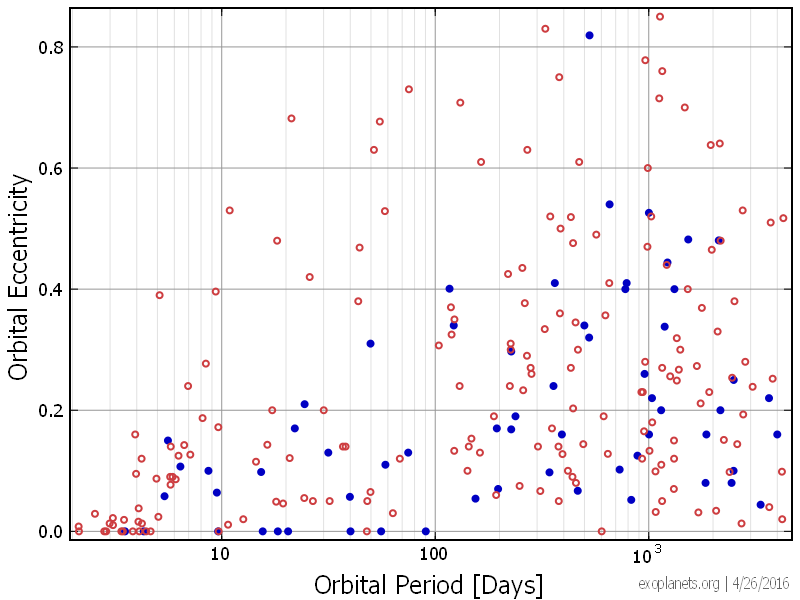
Fig. 1. The eccentricities versus periods of all stars. The eccentricities of orbits of stars more iron abundant than the sun (``iron-rich,'' red open circles) are higher at most all periods than the eccentricities of orbits of stars less iron abundant than the sun (` `iron-poor,'' blue filled circles).
Fig. 2. Eccentricities of the orbits of planets around only stars that are ``sunlike'' in temperature and surface gravity, and in being single stars. Symbols same as Fig. 1. The lower eccentricity at most periods of orbits of stars more iron rich than the sun can be seen, as well as the peaking of the eccentricity of orbits of stars that are poor in iron relative to the sun at periods above 500 days.
 
 Eccentricity as a function of period for selected populations

All and Sunlike:

The eccentricity as a function of period, with whether iron-abundance is poorer or richer than solar indicated, are shown in Fig. 1 for the full and some selections of the 429 orbits of planets found by radial velocity (RV) found with periods of up to 5000 days, followed by Fig. 2 which shows the selection of 243 orbits chosen for stars that are more ``sunlike’’. The ``sunlike’’ sample was selected by taking the 243 planets of the 429 available objects found by RV, where ``objects’’ refers to the set of parameters describing a planet, its star, and their orbit. Stars with different parameters might not have the same features or have them at the same period, so only stars similar to the sun are compared here. Since planet searches have emphasized sunlike stars, this group of stars has the highest number of objects with similar stars available for study. Sunlike objects are those which have stars that have no stellar companion with effective temperatures (or Teff) of 4500 to 6500 K to be close to the Teff of the sun of 5772 K, and with surface gravity not too much less than the sun's value given in logarithmic terms of 4.4. We do not at this time remove stars with very different masses than the sun because not too many remain in this sample, but it may later be important since the small data on lower mass stars could indicate that the peaks and gap feature may occur at shorter periods. Different markers are used to separate orbits by whether the star is poorer or richer in iron abundance than the sun, [Fe/H] <= 0 or [Fe/H] > 0 respectively, shown by the blue filled or red unfilled circles respectively. Table 1 gives the counts in each cut with each cut divided into how many iron-poor and iron-rich objects there are.

Features stand out:
Several features stand out, starting with a broad increase in eccentricity with period at the shorter periods that results from the shortest period orbits having their eccentricities reduced (commonly said to be ``circularized'') due to tidal interaction with the star.  This affects all populations of orbits. When those orbits of stars that have less or more iron than the sun are separated, which are referred to as ``iron-poor'' and ``iron-rich'' objects, it can be seen that the eccentricities of the iron-rich objects rise more rapidly from zero than do the eccentricities of the iron-poor objects, leading to the ``eccentricity-metallicity’’ correlation found between the eccentricity of moderately short period planet orbits and iron abundances found by Taylor (2012, 2013b) and Dawson \& Murray-Clay (2013). This correlation is strongest at periods of roughly 100 days (the ``valley’’ region) but may persist more weakly at periods up to 500 days. The eccentricities of the iron-rich objects have a broader peak, while the eccentricities of the iron-poor objects come more sharply to a peak, and then decline more. The result of the peaking of the eccentricities of iron-poor objects is that the correlation between eccentricity and iron abundance goes away for a middle range of periods from 500 days (shown in Taylor 2013b) upward into the periods where we are showing there is a gap in the number distribution of iron-rich objects. We are preparing work that shows that beyond that gap, the correlation likely returns.

In further work, it will be shown that the correlation of eccentricity is not simply bimodal with iron abundance but the eccentricity changes gradually with iron abundance, that is that the eccentricities of objects slightly above solar have, in periods where the correlation exists, a higher means than iron-poor objects but lower means than for objects with the highest iron abundances.

Fig. 3. Eccentricity versus period of planet orbits of sunlike stars in single-planets, with marker symbols showing whether the iron abundance is above or below solar ([Fe/H] of 0) as in Fig. 1.

Fig. 4. The ''spike'' in the eccentricity of planet orbits of sunlike stars that are in multiple planets systems can be seen clearly here all being between periods of 44 and 75 days. Symbols as in Fig 1. Four of these five are higher than the eccentricity of any other eccentricity. The eccentricity clearly slowly rises with period for both iron-poor and iron-rich stars, though few iron-poor stars are found in multiple systems at longer periods.

Different patterns in eccentricity by period of orbits
 in single-planet versus Multi-planet systems:
In the next two figures the eccentricity versus period is shown for two populations formed by further dividing the sunlike sample of 243 objects. Fig. 3 shows the eccentricities for the 148 ``single-planet’’ objects for which the planet is the only planet found orbiting its host star, and Fig. 4 shows eccentricities for the 95 ``multi-planet’’ objects for which one or more additional planets has been found.

The single-planet sample has a distribution that retains more of the description of the full sample, as this sample has higher mean eccentricities at most periods. This is expected given that the orbits in multi-planet systems are constrained from being too eccentric.
The eccentricities of the multi-planet sample do not peak but continue to rise with period, though the number counts of iron-poor multi-planet objects drops off such that there are far fewer iron-poor multi-planet objects than iron-rich multi-planet objects at periods longer than 1000 days.For multiplanet objects in just sunlike systems there is 1 iron poor vs 23 iron-rich objects at periods longer than 1000 days.

Single-planet and Multi-planet:
We take the 243 sunlike objects separately show the eccentricity versus period distributions for the 148 orbits of ``single-planet’’ objects, or of planets that are the only planet found, and of 95 ``mutiple-planet’’, or of planets for which at least one more planetary companion has been found. The breakdown of counts into iron-poor and rich objects are given in Table 1.

The two distributions look quite different, with the eccentricities of the multiple planets lower in general. This is as expected that a planet is more likely to have a more orderly orbit if there is another planet in the system. The full description of how different these two populations are will be given in upcoming work, while the focus here is on the spike in eccentricity in the multiple planet population. Some qualitative differences besides the spike jump out, including how in the multiple-planet population, the number of iron-poor objects drops off at longer periods. This drop off contributes to the ratio of iron-poor to rich objects being higher for the single planets (40:108 or 0.37) than for multiple planets (23:72 or 0.32).

Whether other than the spike the shape of the eccentricity distributions in the multiple planet population bear a lower eccentricity resemblance to the single planet distribution is a subject of current work. The highest eccentricity point of the iron-poor multiple planet population, HD_192310_c, is at 0.32 much higher than the 2nd highest eccentricity of 0.21 (the 24.451 day HD_7924_d). Its 525.8 ± 9.2 day period fits within the 500 to 600 day period range of the spike in eccentricity of the general population that is the subject of Taylor (2014). While it may be difficult to attach too much significance to one point, it is notable for being such an outlier.

The region of the spike in the eccentricity versus period distribution of the multiple planet population corresponds to a region without similarly high eccentricity objects in the same period range of the single planet population, though if objects that include stars with stellar companions are not cut, there is one such object in this period range of the iron-rich population of the full (not sunlike) selection.

This does raise the possibility that perhaps the spike is simply ``cut out’’ of the single plus multiple planet population by a greater likelihood of finding a planetary companion for planets within this region. This could be true of either physical causes or observational effects. It seems unlikely, though, that the shorter period edge could be a result of not finding companions to shorter period planets. It is worth further work studying this possible effect.


Table 1. Counts of numbers of objects in figures in each cut, with counts of objects divided by whether the abundance of iron of the star is poorer or richer than the sun.
Fig Number
Selection
Total objects
Iron-poor objects
Iron-rich objects
1
All RV objects
429
149
280
2
``Sunlike’’ objects in temperature and surface gravity
243
63
180
3
Single-planet sunlike objects
148
40
108
4
Multiple-planet sunlike objects
95
23
72


Spike Description:

The five planets comprising this spike have orbits with periods from 44 .2 to 75.3 days. Planets orbits tend to be spaced at increasing distances such that it is best to look at planet orbits in ``log space’’ where it is common to give the logarithm to the base 10. When looked at in log period space, this is the very small range of 0.23, going from 1.65 to 1.88 in logarithmic period. This 0.23 is very small given that the range of RV planets that are comparable can be said to have a length of 2.58 in ``log period space’’, going from below 10 days to 5000 days, which is going from log of 1 to log of 3.70. How could planets that are in multiple planet systems have orbits with the highest eccentricities be confined to such a small range?

We must evaluate not only whether this spike could be random or observational, but also whether it could be a result of making the selection of the parameters, especially on making the selection on multiple planet systems. We address how could be possible that planets selecting a part of a larger population, in this case choosing those planets that are in multiple planet versus single planet systems, could have led to a small range in period of planets being preferentially put into this multiple-planet population while planets just outside this range might be preferentially chosen into the single-planet population. It could be the observational effect that planets in slightly longer periods would actually still be in multiple systems but at longer periods that are still too long for them to have been found. A similar explanation would be that there simply are not further planets at the longer periods, but this physical explanation would be of interest as it would be relevant to the existence of peaks in the planet population counted by period.

The presence of high eccentricity orbits in the corresponding period range shortwards of the spike in the single planet system population argues against explanation of tidal dissipation in the star creating the short-period edge of the spike. It also argues against  not having found companions as an observational effect since these companion would not be expected to have longer periods, unless there is a physical reason for the companions not to have been found. It is possible that the longer period companions would have periods within the gap that has been found in the iron-rich population, but that these companion planets are simply ``not present’’ due to the gap.`

Likelihood Section:
Calculations show a low likelihood that high eccentricity orbits would be so close in period

The first questions to ask when seeing an apparent feature must be to determine whether the feature is a real physical feature, starting with asking if the feature might just be a random fluctuation in a small numbers of data points.

The chance that the highest planets in eccentricity would be confined such a small range depends on whether the likelihood is evaluated as being the chance of five high values occurring in the somewhat local range where all five are the highest values, or if the chance of the four highest values occurring over the entire range, but the two give similar results of under one percent and a few thousandths respectively.

The five orbits can be considered to by five pairs of log period and eccentricity values. These are listed below, with the (not log) periods in days preceding each pair for easy reference:

Table 2: Period 
(in days and in base 10 logarithm of the period in days) 
and eccentricity of the five high eccentricity objects.
PER
log period
ECC
day


44.24
1.65
0.47
51.64
1.71
0.63
55.01
1.74
0.68
58.11
1.76
0.53
75.29
1.88
0.73

The calculated likelihood of a certain number of periods occurring within a larger range depends on the length of the range we consider these values might have occurred in. Below we will calculate the likelihood for the five values to be higher in a large part of the full range in period, and then will calculate the likelihood that four values have higher eccentricity than any other object at any period. We choose to be conservative by considering that higher periods are only likely to be larger for longer period orbits, due to the general pattern for eccentricities to get larger with increasing period as a general pattern up to periods of several hundred days. We consider that the eccentricities of shorter period orbits may be lessened by the tidal interaction with the star that tends to circularize the shortest period orbits, so to be conservative, we look for the possibility that these eccentricities randomly occur at some period from shortest period of the spike to one of two longer periods discussed below. It should be noted that in the population of planets without planetary companions, there are high-eccentricity planets by periods of 20 days, so the period ranges given below could have been taken to be longer, even further reducing the likelihoods given below. Looking at the values of eccentricity versus period for single planets shows higher eccentricities for shorter periods in that population, however, leading the values calculated here to give a higher likelihood of this spike resulting from chance, but we choose to err on the conservative side.  In calculating the probability that these periods will occur within the spike range, we take the shortest period of the high eccentricity points, 44.2 days or 1.65 in log-period space, as the shortest period of the range of the periods just as likely to have high eccentricity orbits. The next period at which a higher eccentricity than the lowest of the five occurs is at 567.9 days, or 2.75 in log period space, so these five values could have occurred anywhere along a log period range of 1.11, but they all occurred within 0.23. So the likelihood that five points that could have occurred in 1.11 but occurred in 0.23 can be calculated by finding how often five values appear in the fraction 0.23/1.11=0.21 of points randomly generated from 0 to 1.

Performing random selections of one million sets of five periods from 0 to one shows that only 0.7% of random selections of five values will be within a range of 0.21 of each other. We calculate this by taking the difference between the highest and lowest of the five selected values to allow for the possibility of the five points grouping anywhere within this range. We repeat this procedure to consider how likely is it that the highest four points are within the short range that we find them where we could find them in anywhere up to the full 5000 days for which RV periods are available, or 1.99 in log period from the log values of the period range of 51.6 days to 5000 days. Since the lowest of the five eccentricity values also corresponds to the shortest period, there are now four points from periods 51.6 to 75.3 days, which is 1.71 to 1.88 in log period, spanning a range of 0.16 in log period. This is 0.082 of the 1.99. The chance of randomly having four points within 0.082 randomly generated from points from 0 to 1 is 0.21%. We conclude that this feature is unlikely due to random clustering of the periods at the better than 1% level.

Abundance

The five high eccentricity orbits are characterized by much higher iron abundance in the stars than in the other 15 of the 20 orbits in the full population in the similar period range from 10 to 100 days, reflecting the strong correlation between iron-abundance and eccentricity found in this range. Four of the five have iron abundances higher than all 15 of the stars with low eccentricity planets in this range, and the lowest iron abundance of the five is still higher than more than half of the other 15.

Discussion

Simulations of the likelihood that the periods of the four or five highest eccentricity objects show that the spike is unlikely to be completely random. It is also unlikely to be completely observational effect, but the presence of high eccentricities in a small range of period could be influenced by the interaction between the physical distribution and how additional planets are found.

It is essential to consider whether this spike is merely ``shaved’’ out of the full distribution. The short and long period edges are considered separately. The shorter period edge of the spike could be created by shorter-period orbits having their eccentricities reduced by tidal dissipation. For the longer period edge, there is the possibility that there are higher eccentricity longer-period orbits of planets in systems with more than one planet for which the additional planets have not yet been found so these eccentricity values are still showing in the single-planet plot instead. While both of these possibilities should be researched further, comparison with the single-planet distribution gives some evidence that these are not the explanation for the appearance of a spike. This evidence includes how orbital circularization falls off more quickly allowing higher eccentricities in the single-planet population with periods shorter than 44 days. The single-planet distribution has a rise in eccentricities for periods much shorter than 44 days, and it is more of a gradual rise. It must be noted that the region of the spike shows a possible hole in this region in period space of the high-eccentricity envelope of the single-planet population.

At slightly longer periods, there is a paucity of high-eccentricity systems for both single and multiple planet populations from the range of the spike to over 100 day periods, so there are not enough values there to move over to the multi-planet population. (It is worth noting this paucity that is longwards of the spike, but low statistics makes it uncertain that this paucity is an actual gap feature.)

Does having so many different sources invalidate these results?

It is important to address that the catalog of planet orbits is collected from many different surveys which can have very different efficiencies and standards, which lead many to distrust looking in such a collected dataset for patterns. It is hard to believe that the appearance of these features could be from differences between different observers, especially given how different populations show clearly different patterns that it is improbable that observers could be selecting for. Any observational effects should similarly affect measurements of planets hosted by sunlike or not sunlike stars, and single or multiple planets or stars. For some features to appear so strongly should give confidence that the quality of RV exoplanet data is consistently very high.

Further observations to lead to further work:

It appears that, other than the spike, the shape of eccentricity distribution by period of iron-poor and iron-moderately-high multiple planets appears to be a ``pushed down’’ version of the single planets distribution. Future work must address whether both the iron poor objects in the full population and the iron poor objects in the multiple planet population have a similar spreading of the spike with increasing iron abundance in the range  0 < [Fe/H] < 0.1 of the in eccentricity that occurs in the 500-600 day range.


The finding of a spike in eccentricity in the population of planets with planetary companions again shows that pattern formation and evolution leads to more uniform distributions than expected. The presence of distinct features in the eccentricity and number distribution by period shows that the evolution of planets which could include activity such as planet scattering after formation that could smooth out these patterns, is likely not to overly disturb patterns that occur in system after systems.

These results suggest that the pattern of planet formation is like more predictable and less random from one planet system to the next. The presence of these features prompts the suggestion that observers of protoplanetary disks (PPDs) look for whether the rings and gaps in PPDs tend to have repeating patterns from disk to disk, or if the features now being found in PPDs tend to be found at random periods. The preservation of features in the number and eccentricity distribution presents the opportunity to learn about planet formation through studying features found in the parameters of mature planet systems.